# Backend
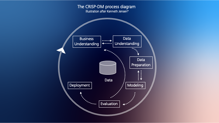
The following documentation is structured after the CRISP-DM process.
NOTE: For the first step in the CRISP-DM, visit the Design Thinking and Process page and for the second step the Data Source section.
# 3. Data Preparation - Speed Layer
The following paragraph will focus on the data preparation and aggregation as it is performed in the speed layer. This closely represents the Data Preparation phase of the CRISP-DM approach. However, it does not cover the process for selecting relevant variables during development of the solution. A few remarks on this step will be given after the documentation of the speed layer.
# Input
The Speed Layer processes the simulation-data which is consumed from a Kafka-Stream. After parsing the JSON-data, it gets converted to a pyspark-DataFrame (pyspark.sql.DataFrame).
df = spark.readStream.format("kafka") \
    .option("kafka.bootstrap.servers", "kafka:9092") \
    .option("subscribe", "simulation") \
    .load()

df = df.selectExpr("CAST(value AS STRING)")

df = df.withColumn("value", from_json("value", schema)) \
    .select(col('value.*')) \
# Transformation
In the transformation phase, the data goes through several steps: Filtering, Harmonization, Aggregation, Enrichment. The Filtering- and Harmonization-Phase are less needed due to the fact that most of the data comes from the same simulated data source and is pretty much homogeneous. For real world data, this processing step would have to be extended.
# Aggregation
The incoming data-stream gets aggregated by each trip.
- Master-data (such as the corresponding route, truck or trip) is saved once.
- Moving-data is converted to time series. This enables the resource efficient historization of the data for later use in the Batch Layer. The time series are of use for computing metrics like averages, moving averages (not implemented in the latest version), standard-deviations (not implemented), and for deriving most recent values, which are used in the frontend.
- As mentioned above, moving data for which only the last value is of relevance to the frontend is saved in a separate field to be forwarded to the frontend api. Some constantly changing values which are not of importance for machine learning (such as the weather, which currently has no influence on the simulation) are treated the same way to save on resources. In a production environment, it would be a good idea to save everything to the batch database in case this data is needed in the future for different use cases.
An example of all three aggregation types:
df_serve = df_serve \
    .groupBy('tripId') \
    .agg(F.first("truckId").alias("sd_truckId"), \
    F.collect_list('speed').alias("ts_speed"), \
    F.avg('consumption').alias("agg_last_consumption"))
# Enrichment
Additional master-data is joined, such as the length of each route, to compute metrics like the current progress per trip. The length of each route is a static dataframe that does not require recomputation in the batch-layer. Rather, this dataframe would have to be updated by a route planning system as soon as a new route is entered into the system.
AS.download_file(save_path, cloud_file_name, container_name)
route_dist_pd = pd.read_csv("./route_dist.csv")
route_dist = sqlCtx.createDataFrame(route_dist_pd)
df_serve = df_serve.join(route_dist, 'sd_routeId', how='left_outer')

@udf("array<integer>")
def PRODUCE_ts_agg_acc_meters(xs):
    if xs:
        temp = [int(round(sum(xs[0:i]), 0)) \
        for i in (range(1, len(xs) + 1))]
        return temp

df_serve = df_serve \
    .withColumn("ts_agg_acc_meters", \
    PRODUCE_ts_agg_acc_meters("ts_meters_intervall"))
Historical aggregates, stemming from the Batch Layer, are used to compute Delta-KPIs. Those fulfill the purpose to better assess current data, when seeing it in relation to values which can be considered normal for each route. For this, similar to joining master data above, aggregation data is joined and then used set current values into comparison. The aggregations are periodically recomputed by the batch layer to ensure that averages are up to date.
External datasources, such as the current weather for each truck, get joined as additional data for the frontend. A custom weather api caller was defined in order to obtain weather codes in concordance with the frontend specification. Additional information, such as a description of the weather, the temperature or humidity would also be available.
@udf("integer")
def get_weather_code_for_location(lat, lon, unix_time):
    result = Weather.get_weather_for_location(lat, lon, unix_time)
    return result[0]

if (enrich_weather_data):
    try:
        df_serve = df_serve \
            .withColumn("weatherCode", \
            get_weather_code_for_location("lat","lon","timeStamp"))
Machine Learning Models are used as inference-engines, to enrich the streaming data with predictions, such as the delay per trip. The models are fetched from Azure Blob Storage. A simplified code fragment showing the general process:
newest_filename, s = AS.get_newest_file(container_name, arrival_file_substring)
filepath, s = AS.download_file(save_path, newest_filename, container_name)
arrival_model_path = AS.unzip(".", filepath)
model_arrival = PipelineModel.read().load(arrival_model_path)
df_serve = model_arrival.transform(df_serve)
# Output
There are two outputs of the Speed Layer. A subset of all features (mostly aggregates such as averages or last values and identifying labels) get forwarded to the frontend via an Kafka-Stream.
df_to_frontend_stream = df_to_frontend \
    .writeStream \
    .format("kafka") \
    .option("kafka.bootstrap.servers", "kafka:9092") \
    .option("topic", "frontend") \
    .outputMode("Complete") \
    .option("checkpointLocation", False) \
    .start()
A sample of one message to the frontend:
{"trip_id":"VA1Z9OT98P","truck_id":"5f070922c92647260c2b2886","number_plate":"S HZ 8245","route_id":"5f070922c92647260c2b287e","truck_mass":14070,"departure":"Muenchen","arrival":"Stuttgart","departure_time":1595456465,"telemetry_timestamp":1595456465,"arrival_time":1595466901,"telemetry_lat":48.16400894659716,"telemetry_lon":11.483320377669836,"truck_speed":13.08,"truck_consumption":6.66,"avg_truck_speed":13.08,"truck_acceleration":-6.07,"avg_truck_acceleration":-6.07,"normal_consumption":6.66,"route_progress":0,"driver_class":1,"delay":-1773,"driver_acceleration":2,"driver_speed":2,"driver_brake":0,"incident":false,"truck_condition":1,"tires_efficiency":0,"engine_efficiency":0,"weather":0,"year":2008,"arrived":0,"truck_type":"LOCAL","driver_duration":0,"road_type":"INTERURBAN","next_service":212,"service_interval":9000}
Secondly, all master data along with all time series is saved to the batch layer, by inserting it into the persistence-layer (Cosmos-DB) in a historized fashion. We decided to insert the already preprocessed and enriched data into the batch-db (and not directly from the simulation) to ensure consistency in terms of enrichment steps. Therefore, the foreachBatch()-Method was used, in order to insert data via the pymongo library.
def write_to_mongo(df_to_batch, epoch_id):
    tempdataframe = df_to_batch.toPandas()
        with pymongo.MongoClient(uri) as client:
            mydb = client[mongodb_name]
            sparkcollection = mydb[mongodb_collection]
            df_json = json.loads(tempdataframe.T.to_json()).values()
            try:
                sparkcollection.insert(df_json)

df_to_batch_stream = df_to_batch.writeStream \
    .outputMode("Update") \
    .foreachBatch(write_to_mongo) \
    .start()
A major hurdle was inserting the label for time series into the database. The dependent variable for the estimated delay prediction is calculated using the accumulated amount of seconds per trip. This value is only available with the last signal for each trip, as soon as a truck has arrived at its destination, but has to be inserted for all previous tuples of the corresponding trip, which have already been saved to the database at that point. Updating the documents in the batch-db has to be done to allow the training of models, eligible of predicting the label for each step of the time series.
sparkcollection.update_many( \
	        {"tripId": temp_tripId}, \
		    {"$set": {"LABEL_final_agg_acc_sec": temp_LABEL}})
As the data stems from a simulation, data cleaning did not have to be performed. However, a large problem that was faced during development was the constantly changing nature of the data, as the development of the simulation was simultaneous to the development of the backend. It would have been better to have a fixed data source from the start. This would have enabled structured work, more consistent with CRISP-DM.
# 4. Modeling - Batch Layer
In the modeling phase, we ended up with two models. One supervised, and one unsupervised approach.
We clustered the driver-habits using the spark-proprietary K-Means-Clustering-Algorithm and evaluated the models with Silhouettes. Incremental-Model-Training / Online-Training was considered for the clustering, but could not yet be implemented.
CL_kmeans = KMeans() \
	    .setK(3) \
	    .setSeed(1) \
	    .setFeaturesCol("scaledFeatures")
Gradient Boosted Trees (GMT) were utilized to regress on the delay per trip and evaluated using the Mean Absolute Error.
EA_gbt = GBTRegressor(labelCol="label", featuresCol="features")
The GBT-Algorithm was challenged against LSTM-Networks, which held the potential to make better use of Time Series Data. However, while the data is available in time series format, the prediction is a regression task and heavily profits from the ability of GBT to learn different patterns in data. Unfortunately the LSTM, implemented with Keras and Tensoflow as Backend, was not able to achieve better results than the sequentially growing decision trees. In the next iteration of the data science process, it could be tried to predict the delay using a multi model or multi input model approach with LSTM's and dense networks, concatenating several input streams with different dimensionality. This would not only process time-series, but also one-dimensional master data, which turned out to be a good predictor with the GBT. Anyway, the LSTM code can be found here.
For both models, the hyperparameters were optimized with the help of a Grid Search. The grid could be extended by further variables if better results are required, it is however more likely that training data amounts and data preparation play a bigger role in the quality of the models.
EA_paramGrid = ParamGridBuilder() \
        .addGrid(EA_gbt.maxDepth, [3, 5, 7]) \
        .addGrid(EA_gbt.maxIter, [10, 20, 50, 100]) \
        .addGrid(EA_gbt.stepSize, [0.001, 0.01, 0.1, 1]) \
        .build()
# 5. Evaluation
# Evaluation of Machine Learning Models
Each parameter combination in our grid is evaluated using 10-Fold-Cross-Validation, due to the fact that is an sufficiently big and decorrelated estimate of our error-metric.
EA_pipeline=Pipeline().setStages([EA_indexer1,\
			    EA_indexer2, \
			    EA_vectorAssembler, \
			    EA_gbt])

EA_crossval = CrossValidator(estimator=EA_pipeline, \
                          estimatorParamMaps=EA_paramGrid, \
                          evaluator=RegressionEvaluator(), \
                          numFolds=10)

EA_crossval = EA_crossval.fit(sql_df_trips)
EA_best_model = EA_crossval.bestModel
Lastly, we found heteroscedasticity in our prediction-error, meaning that the variance of our error-estimate was not constant. We were not able to eliminate this issue yet.
jointplot= sns.jointplot(x="label", \
		    y="pred", \
		    data=sql_df_trips)
# 6. Deployment
NOTE: For a detailed description of how to deploy Horizon yourself, please see the tab How to deploy.
Before beginning work on Horizon, Microsoft Azure was chosen as the platform on which it would later be deployed. This is for two reasons: Firstly, Azure is currently shaping to be the main competitor to the industry leading Amazon Web Services and offers a free student credit program, making it well suited for a study project. Secondly, while some team-members had previous experience with Googles Cloud Platform, another option with a student credit offering, we wanted to gain experience with another solution.
We did not expect that hosting our solution would require many resources, but in the end the student credit of multiple accounts was fully used up, also due to experimenting with different features.
Azure Kubernetes Service and Azure Cosmos DB were chosen early in the process as the two main components on which Horizon runs. Subsequent architecture and tool decisions were made accordingly.
After testing parts of the solution in clusters or containers on local machines, the live deployment only required small changes to the general workflow, the largest being heavy wait times while waiting for container images to upload for live testing.
As Horizon was developed as a prototype and underwent constant changes, in addition to the high cost of hosting the service, Horizon did not run online for extended periods of time. This means that no large database of data for training could be collected. Monitoring was therefore not required (and would have cost additional credit). The Batch Database did not reach full capacity and remained below the free tier of 400 RU/s for the duration of the project.
# Contributors
David Rundel and Felix Bieswanger were mainly involved in the development of the backend and streaming. Jan Anders helped with deployment.