# Data Source
Welcome to the official documentation of the Data Source of Horizon - an extended fleetSim.
# The search for a viable data source
Firstly, a data source had to be found which delivers realistic and arbitrary amount of real time streaming data of a truck fleet. FleetSim was found to be a suitable base simulation which could be extended to deliver the required data fields and amounts.
The original fleetSim simulation was extended in three important ways:
- Important variables, physical and random effects were added to make the simulation more realistic.
- Each simulated truck is able to stream updates of its movements to a kafka server.
- A large endless simulation that only runs on predefined routes was created.
Before describing the data the simulation delivers, a detailed description of the first and most important extension is provided.
# Extending FleetSim
Further research is necessary for the extension of FleetSim. It is important to find values that influence the real consumption of a truck and by which core variables can be described. It is also necessary to be able to simulate the behaviour of a real driver and the current technical condition of the truck.
In the following, the results of the research and the implementation in the simulation are shown.
# Simulation of the truck
The trucks are already implemented in the simulation but only on a very basic level. With expanding the truck variables the simulation becomes more realisitic. Beforehand it is neccessary to define which variables of a truck influence the overall consumption.
The engine of a truck converts the chemical energy from the fuel into mechanical energy that makes the truck drive. The greater the efficiency and the less energy is lost through external influences, the more fuel-efficent the truck drives.
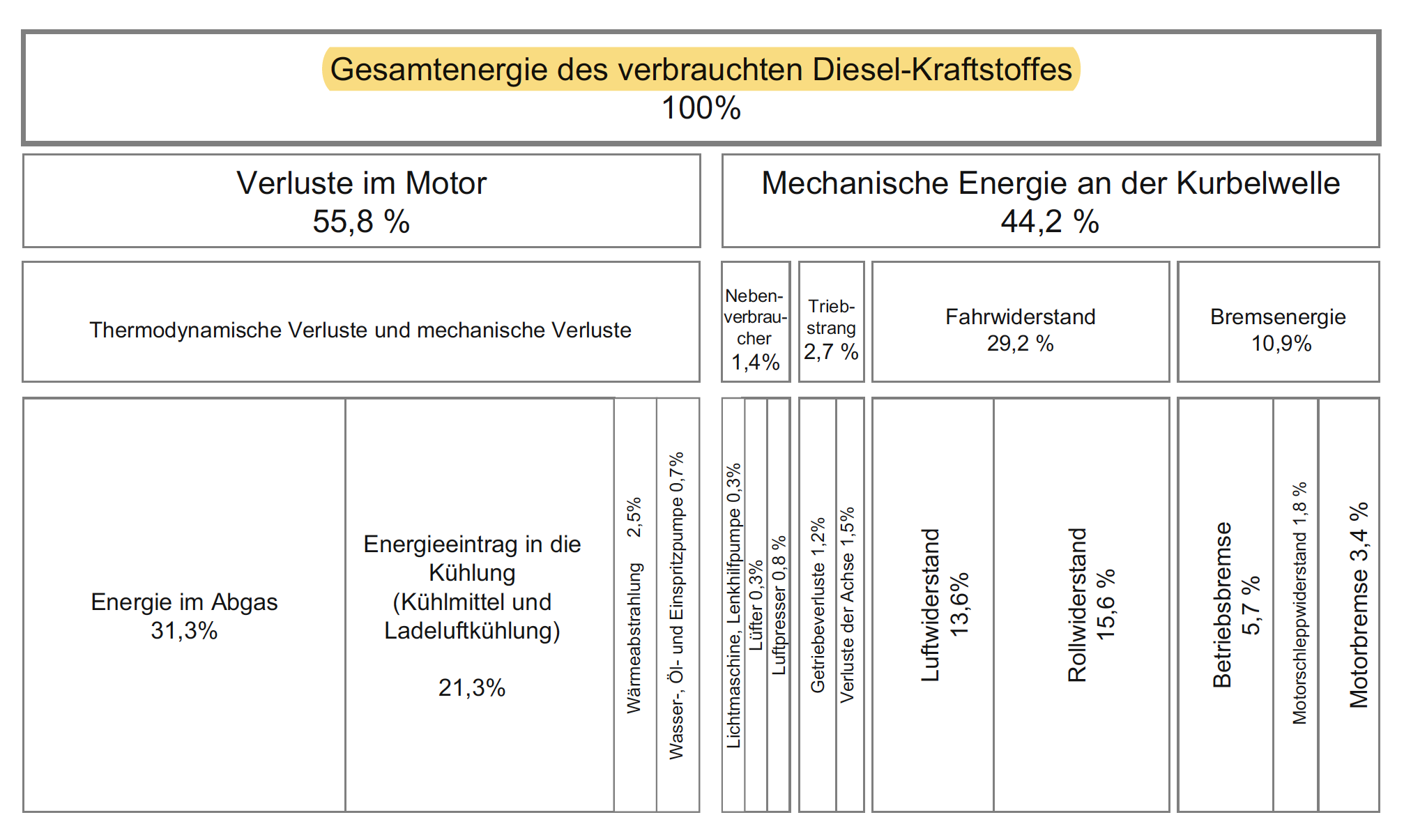
Accordingly, it is important to know which parameters influence the efficiency. Hilgers, 2016, breaks down the energy losses as follows:
 Imagesource: Hilgers, 2016, p. 8.
Beside the energy losses in the engine, which can hardly be influenced, the losses due to mechanical energy at the crankshaft are relevant for further calculations. The greatest variable here is the rolling resistance of the vehicle - i.e. all forces that brake the vehicle and which must be overcome. These include rolling resistance, air resistance and gradient resistance. (Hilgers, 2016, p.9). This force has to be balanced to keep the speed constant or to overcome it in order to accelerate. The factors mentioned, such as the alternator, fan, transmission, axle or engine brake, are largely dependent on vehicle technology.
Besides vehicle technologie the vehicle model itself has a major impact on the consumption. Depending on weight, overall dimensions and frontal area, consumption changes significantly.
To simulate everything, the following variables were implemented:
# Truck identification
Basic truck information for identification purposes:
	this.id = id;
	this.licensePlate = licensePlate;
# Truck type and year
Truck type and age massively influence the consumption and technical condition of the truck.
this.truckType = TruckType.from(truckType);
In the simulation, three different truck types were defined:
- local
- long_distance
- long_distance_trailer
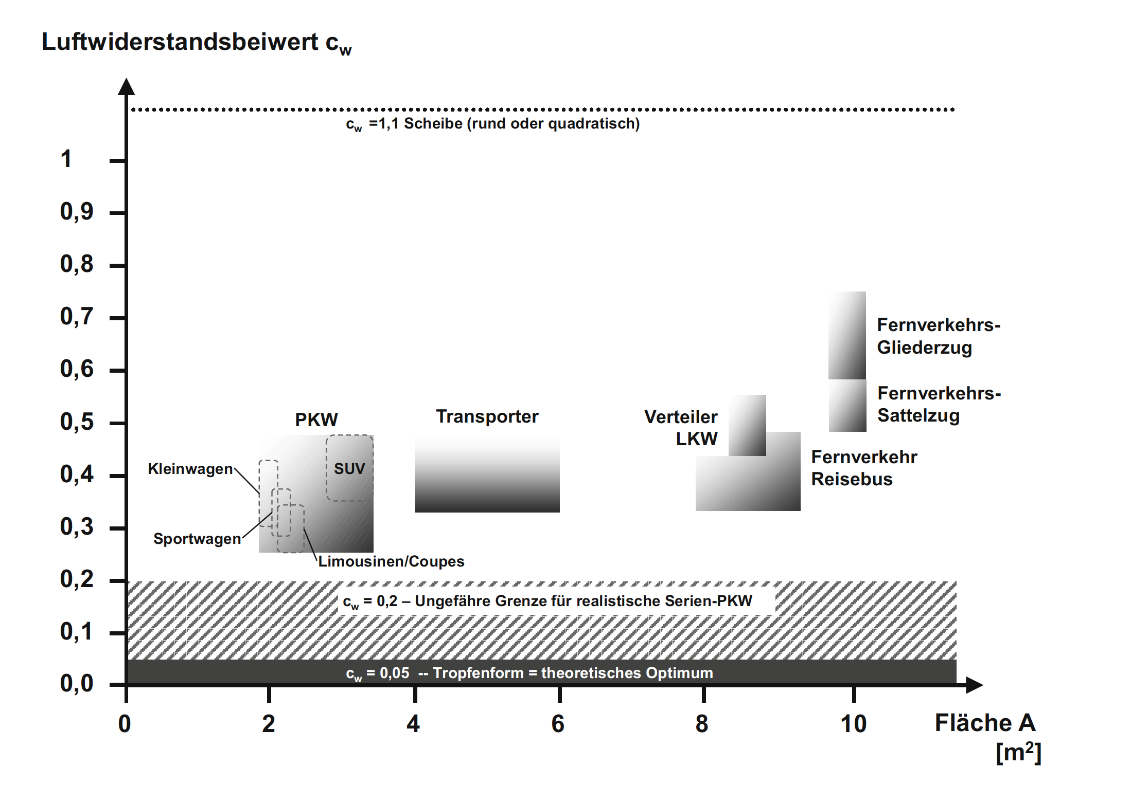
Each of the different truck types has different values for the truck front surface and therefore for the drag coefficient. All used values are illustrated and defined in Hilgers, 2016, p. 19:
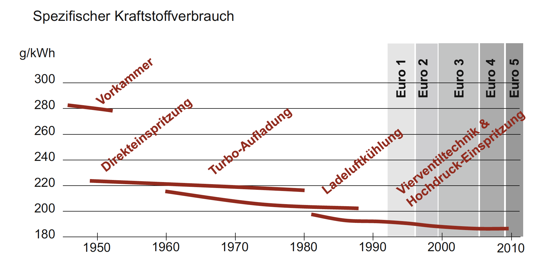
The calculation of the drag coefficient is also described in Braess & Seiffert, 2013., p. 50. The age of a truck has also an impact on the overall consumption, as technical features improved over time: "So konnte der Verbrauch von vollbeladenen 40-Tonnern zwischen 1965 und 1995 um circa ein Drittel gesenkt werden" (Hilgers, 2016, p. 11). The truck simulation was extended by four different age intervalls with random possible fuel consumption values for each year intervall:
/** Returns specific fuel consumption in g/kWh based on model year */
private double getRandomSpecificConsumption(int year) {
	double efficiency1990 = GenerationHelper.getRandomValue(191.0, 195.0);
	double efficiency2000 = GenerationHelper.getRandomValue(187.0, 189.0);
	double efficiency2010 = GenerationHelper.getRandomValue(184.5, 185.5);
	double efficiency2020 = GenerationHelper.getRandomValue(182.5, 183.5);

	if (year >= 1990 && year < 2000 ) {
		return efficiency1990 + (year-1990) * (efficiency2000 - efficiency1990) / 10;
	} else if (year >= 2000 && year < 2010 ) {
		return efficiency2000 + (year-2000) * (efficiency2010 - efficiency2000) / 10;
	} else if (year >= 2010 && year < 2020 ) {
		return efficiency2010 + (year-2010) * (efficiency2020 - efficiency2010) / 10;
	} else {
		return 0;
	}
}
	this.year = year;
The source for those intervals can be found in this illustration from Hilgers, 2016, p.12:
# Truck mass and payload
Truck mass and payload are an important value as they are influencing the consumption. The higher the total mass of a truck, the higher the needed energy (fuel) to overcome to overcome the inertia:
	this.massEmpty = massEmpty;
	this.massPayload = getRandomPayload(this.truckType, this.massEmpty);
The mass is dependant on the truck type and a random payload. The maximum payload is the maximum allowed payload for each truck type. All information on the maximum permitted upper limit can be found here and here
private int getRandomPayload(TruckType truckType, int massEmpty) {
	int massPayload = 0;
	if (truckType == TruckType.LOCAL) {
		massPayload = GenerationHelper.getRandomValue(0, 18000-massEmpty);
	} else if (truckType == TruckType.LONG_DISTANCE) {
		massPayload = GenerationHelper.getRandomValue(0, 26000-massEmpty);
	} else if (truckType == TruckType.LONG_DISTANCE_TRAILER) {
		massPayload = GenerationHelper.getRandomValue(0, 40000-massEmpty);
	}
	return massPayload;
}
# Truck condition
The truck condition also has a major impact on the consumption of a truck. To make the simulation not too complex and give attended data processing algorithms the possibility to identify all three influences, factors are chosen which lineary incfluence parts of the consumption formula. All of the three values range from 0% which equals "bad condition" and 100% which equals "best condition". The truck condition will influence the general factor for the moment of inertia of all rotating masses. This is because e.g. bad oil or worn bearings will increase the needed energy to move the masses inside the powertrain. The truck condition gets worse over the time (not the driven distance, to also include traffic jams better). The engine condition influences the final consumption directly by increasing it up to 20%. This shall reflect real defects on the engine, like damaged turbo charger, defect lambda sensor, air mass sensor. While the truck condition changes its initial value slowly over time, the engine condition can change randomly with a higher rate. The tires efficiency is dependent on the currently mounted tire type and covers a wide range of efficiencies of different tire manufacturers (Reithmaier et. al, 2000, p. 37).
	this.truckCondition = GenerationHelper.getRandomValue(0.0, 1.0);
	this.engineCondition = GenerationHelper.getRandomValue(0.8, 1.0); // should not start with a damaged engine
	this.tiresEfficiency = GenerationHelper.getRandomValue(0.0, 1.0);
# Overall simulation of the consumption
Summed up, the consumption of an truck is highly dependant and influenced by many different variables which lead to an extensive calculation. The main source and formula was based on Hilgers, 2016, p. 9 ff and Braess & Seiffert, 2013.
public double getConsumption() {
	double g = 9.81; // m/s^2
	double rho = 1.293; // kg/m^3
	double croll_min = 0.0045; // %
	double croll_max = 0.0065; // %
	double croll = croll_min + (croll_max - croll_min) * (1.0 - tiresEfficiency); // %
	double slopeAngle = 0; // rad
	double frot = 1.1 + 0.4 * (1.0 - truckCondition); // %
	double br = 0; // N
	double a = acceleration; // m/s^2
	double v = speed; // m/s
	double dt = interval; // s
	int massTotal = massEmpty+massPayload;
g: For the gravitational force equivalent is a constant value of 9.81 m/s^2, as it is the value for central Europe.
rho: Rho describes the air density and is valud with 1.293 kg/m^3 (Temperatur: 0° and Pressure 1013hPa)
croll: consists of croll_min and croll_max and describes the rolling resistance factor and is dependand on the tires efficency. More about the tires efficency is described below.
slopeAngle: Always 0 as OSM doesn't provide information about height and slope
frot: a factor which includes the moment of inertia of all rotating masses, is dependant from the truck condition
a: Acceleration
v: Speed
dt: update time
  double maxEngineDefectFactor = 0.2; // %
  double specificConsumption = this.specificConsumption;
  specificConsumption = specificConsumption * (1.0 + (maxEngineDefectFactor * (1.0 - engineCondition)));
maxEngineDefectFactor: Value which influences the consumption if an engine defect occurs
specificConsumption: Dependant on maxEngineDefectFactor and current engineCondition
  double FAir = 0.5 * rho * v * v * surface * cw; // kg*m/s^2
  double FRoll = massTotal * g * croll * Math.cos(slopeAngle);
  double FMountain = massTotal * g * Math.sin(slopeAngle);
  double FAccel = massTotal * a * frot;
  double FTotal = FAir + FRoll + FMountain + FAccel + br;
The calculation and formulas for the different running resistances can be found in Hilgers, 2016, p. 9 ff and Braess & Seiffert, 2013, p. 51 & 52.
	double pEngine = FTotal * v * dt; // Ws
	pEngine = pEngine / 3600000.; // kWh

	double consumption = (pEngine * specificConsumption) / (v * dt); // g/m
	consumption = (consumption * 100.) / fuelDensity ; // l/100km

	consumption = Math.max(consumption, 0.0);
	return consumption; }
# Impact of the speed and road
The OSM calculated route sections have an estimated average velocity for normal passenger cars. The truck simulation always tries to reach this velocity, if it is not larger than the usually allowed maximum speed for trucks of 80 kph. As information for post-processing algorithms, road types are estimated for the average velocities. Four different Route-Types and according speed limits are defined within the simulation:
- URBAN(0):
- INTERURBAN(1): > 40 kph
- HIGHWAY(2): > 65 kph
- FREEWAY(3): > 100 kph
The truck follows a motion model (Intelligent Driver Modell) to reach the OSM estimated average speed (target speed) over time, instead of jumping directly to the speed of a newly entered route section. It also includes the reaction on traffic jams, when the target speed is reduced to 5-30 kph. To achieve this, two speed controllers are used. One is trying to reach the target speed of the current route segment. The other is trying to reach the target speed of the next route segment, if it comes closer. (cf. Treiber, 2007, p. 78)
# Impact of the driver
The driver and his driving style also influence the consumption of the vehicle. At the same time, however, poor driving style could also result in speeding tickets and thus shall be avoided. Since a real driver does not always drive equally well, drivers have a driving style in the simulation. There are four parameter groups defined to simulated this behaviour. Each of the groups can have an overall rating of bad, conspicious and normal driving styles.
- Driver Speed
- Driver Acceleration
- Driver Brake
- Driver Tired
A bad driver speed behaviour leads to driver faster than the OSM has estimated for the route sections and it results to overriding the maximum speed of 80 kph. A bad driver acceleration behaviour leads to higher accelerations with higher rates of change, as well as a later release of the gas pedal, if a new higher speed shall be reached. A bad driver brake behaviour leads to higher deceleration with higher rates of change, as well as a later release of the brake pedal, if a new lower speed shall be reached. The driver fitness influences the ability of the driver, to drive a continuous velocity. To achieve this, a sinus with low frequency is applied on the current target speed. If the driver gets tired, he will deviate more from the target speed in positive and negative direction. If he is fit, he is able to keep the target speed.
# Description of the data
A typical message from the simulation to the kafka server looks like this:
{"truckCond":1,"timeStamp":1595455986000,"speed":13.05292451466845,"avgIntervSpeed":10.38730585107233, "secSinceLast":120,"acceleration":1.5121130926381294,"bearing":315.8724852614906,"mass":27636.0, "consumption":11.251371489442374,"lat":51.05354230592819,"lon":13.724075328077138,"engineEff":0, "tireEff":0,"truckYear":2014,"truckType":2,"speedWarn":0,"accWarn":1,"brakeWarn":0,"incident":false, "routeId":"5f070923c92647260c2b28e9","tripId":"278JHYXZAW","truckLP":"S HZ 9831", "truckId":"5f070923c92647260c2b28f1","roadType":1,"arrived":0}
We can see that there are a few data points which help to identify a record. Such are:
- truckId (and truckLP - license plate)
- routeId
- tripId
- timeStamp
Most data points deliver updates on the state the truck is in. Examples for this are:
- truckCond
- lat and lon (latitude and longitude)
- acceleration
# Data amounts and format
The simulation can run at arbitrary speed and can send messages in custom time intervals. There are therefore two settings controlling the amount of messages which are received from the simulation. The amount of milliseconds in real time that are required to pass for one second in the simulation and the message interval in which trucks send in seconds. Assuming an interval of 120 seconds with the simulation running in real time, this means that on average, a message from a truck is received every two seconds.
Variables providing information on the state the truck or its components are encoded in a three tier system:
- 0: normal status
- 1: conspicuous status
- 2: bad status
Identifying information is mostly delivered as string. Most other variables are provided in numeric format such as the coordinates, timestamp (unix time) or consumption. The speed in provided in m/s.
# Data Exploration
As the focus on the project lied on live streaming data to a dashboard, data exploration was mainly carried out to ensure data quality and consistency.
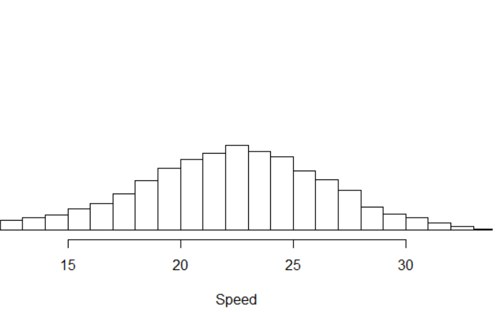
For a simulation with many trucks and a sufficiently large time-frame of multiple days it was found that moving variables such as speed and acceleration are normally distributed.
 It was also found that trucks send their data in reliable intervals and stay on their assigned routes (duh). They commence to a different destination after a random delay (driver gets a break).
# Deploying the Horizon Data Source
# Disclaimer
Apart from the extension of the simulation and adding streaming capabilities and an additional simulation mode, changes were made to fleetSim in order to make the deployment inside DockerContainers feasible. These customizations may have heavily altered aspects of fleetSim which are not required by Horizon. The only purpose of the simulation inside the Horizon system is to endlessly generate telemetry data on known routes with known trucks, or in other words, to simulate the movements of a truck fleet of a logistics company as closely as possible. Other simulation modes are not used by fleetSim and may not run as intended in the current state of fleetSim. Knowledge of the original fleetSim is strongly recommended if this version shall be further developed for other use cases.
# Setup
Installation requirements for fleetSim:
- Java > 1.8
- maven >= 3.3
- Access to a mongoDB >= 3.2
Make sure JAVA_HOME is set on the fleetSim host and mongoDB is running.
The initial setup/bootstrap of fleetSim in order to obtain a compatible mongoDB database requires extensive system resources. For the setup of the simulation for Horizon, an osm file for Germany is required (e.g. from here) and has to be located inside the osm folder.
When first set up on a local machine, the simulation tries to execute a mongoimport command on the host machine, assuming that a mongoDB is running on localhost. If this is not the case, as when the simulation runs in a container, this mongoimport has to have been executed manually to import the collection cities, which are required for route calculations.
The mongoimport was disabled inside fleetSim as it is not needed for the purposes of Horizon after an initial setup of the database.
To initialize the database and calculate routes using GraphHopper, run
mvn compile exec:java@bootstap
This can require some time to execute while GraphHopper first initializes. On a decent computer in 2020, the first bootstrapping phase required 20 minutes while producing timeout messages. There is no indication of when the bootstrapping phase finishes. Laptops or virtualized environments could require significantly more time.
For deployment, it is advisable to only run the initialization phase once on a local machine and save the files GraphHopper requires inside the fleetSim container/host system if dynamic route calculations are needed. Horizon relies on precalculated routes which are stored inside the mongo database. If new routes are needed, this only requires updating the database image, instead of including route calculation logic and large GraphHopper files inside the fleetsim image. FleetSim itself does not require the osm file or an initialized GraphHopper to run, as long as precomputed routes are used.
Once the mongoDB has been setup and the bootstrapper run, the simulation server can be started with
mvn exec:java@run
Alternatively, the simulation can be converted to a .jar and run by any JVM.
From here, the instructions in How to deploy can be followed.
The most important settings that are required during operation can be set inside conf.json. Some considerations on the conf.json that are new to this version of the simulation:
- When seperating simulation and mongoDB, the usingDocker argument should be set to true. This prevents errors when the program tries to load GraphHopper. All functionality that enables endless simulations using dynamic calculation of new routes on the spot has been manually disabled and is not affected by this.
- Streaming to kafka can be turned on/off alltogether by setting the "postData" argument
# Contributors
Anja Stütz and Jan Anders were mainly involved in the development of the data source.
# References
- Braess, Hans-Hermann; Seiffert, Ulrich (Hrg) (2013): Vieweg Handbuch Kraftfahrzeugtechnik. Springer Verlag. DOI 10.1007/978-3-658-01691-3.
- Hilgers, Michael (2016): Kraftstoffverbrauch und Verbrauchsoptimierung. Springer Verlag. DOI 10.1007/978-3-658-12751-0.
- Reithmaier, Walter; Kretschmer, Stefan; Savic, Branislav (2000): Ermittlung von Rollgeräusch- und Rollwiderstandsbeiwerten sowie Durchführung von Nassbremsversuchen mit Nutzfahrzeugreifen. Forschunggsprojez im Auftrag des Umweltbundesamtes FuE-Vorhaben Förderkennzeichen 299 54 114. Umwelt Bundes Amt. Online available: https://www.umweltbundesamt.de/sites/default/files/medien/publikation/long/3261.pdf.
- Treiber, Martin Dr. (2007): Verkehrsdynamik und -simulation. Published script, Institut für Wirtschaft und Verkehr, Technische Universität Dresden.